BigQuery Data Warehouse Best Practices

8 min readJun 17, 2024

What is a Data Warehouse?

A data warehouse is an OLAP solution widely used for organizations where the data from the sources are cleaned and transformed in staging area, before being loaded here for reporting and data analysis. Taking a step further, the data processed in the data warehouse can be served into Data Marts, which are smaller database systems that are used for different teams within an organization as shown in the flow chart below

What is BigQuery?

BigQuery is a serverless data warehouse solution offered by Google Cloud Platform The organization doesn’t need to take care of the infrastructure that processes the data, and offers a relatively fast service in reporting within an organization. Below are some key features of BigQuery

Serverless. There are no servers to be managed or database software to be installed by the organization itself.
The software and the infrastructure itself are scalable and in high availability.
It includes built-in features that support machine learning, geospatial analysis and business intelligence.
It maximized flexibility by separating the compute engine and storage that stored your data.

Pricing in BigQuery

In general, pricing in BigQuery is composed of two main components, which are compute pricing and storage pricing. The details pricing information can be found on the Google Cloud website. In regards to this, it is rather important to have a deep understanding of the organisation's needs and select the right pricing models. You don’t want to waste your money and resources.

The compute pricing models can be classified into two:

On-demand pricing (per TiB). You’re charged for the number of bytes processed by each query. The first 1 TiB of query data processed per month is free. To date, the pricing is $6.25 per TiB.
Capacity pricing (per slot-hour). You’re charged for compute capacity used to run queries, measured in slots (virtual CPUs) over time. This model takes advantage of BigQuery editions, which are the standard, enterprise and enterprise plus editions.

Storage pricing then can be divided into two classes as well, the active logical storage ($0.02 per GiB per month) and long-term logical storage ($0.01 per GiB per month).

An approximation of the size of the data being processed will be shown in the right corner of the window prior running running queries on BigQuery. It might give you a glance at how many bytes of data will be processed by the particular execution. The actual amount of processed data will then appear in the Query results panel in the lower half of the window. It might be helpful to quickly calculate and optimise the cost of the query for your project.

Creating an external table in BigQuery

BigQuery supports external data sources, although the data is not stored in the BigQuery storage. For instance, it can be directly queried from data stored in Google Cloud Storage upon the creation of the external table.

An external table is a table that functions like a standard BigQuery table with table schema stored in BQ but the data itself is external. No preview of data is available in that sense. You might create an external table from a .csv or .parquet file from Google Cloud Storage in this way:

-- Creating external table referring to gcs path
CREATE OR REPLACE EXTERNAL TABLE `de-zoomcamp-412301.ny_taxi.external_yellow_tripdata` 
OPTIONS ( format = 'parquet',
    uris = ['gs://module-3-zoomcamp/yellow/yellow_tripdata_2020-*.parquet',
    'gs://module-3-zoomcamp/yellow/yellow_tripdata_2019-*.parquet']);

Be aware that the estimation of bytes of data for the query from an external table is not available. In regards to that, you can import an external table in BQ as a regular table. For example:

CREATE OR REPLACE TABLE `de-zoomcamp-412301.nytaxi.yellow_tripdata_non_partitoned` AS
SELECT * FROM `de-zoomcamp-412301.nytaxi.external_yellow_tripdata`;

Partitioning

The BigQuery table can be partitioned into smaller tables which improve the query performance, thus saving cost. For instance, if we often query the data by date, we then can further partition our table by date, hence we can do a sub-query based on the date we are particularly interested in. In general, you can partition a table by:

Time-unit columns like Timestamp, Date or DateTime columns in a table
Ingestion time. The timestamp where the data is ingested to BigQuery
Integer range partitioning
The default partition is daily wile using time unit and ingestion time. It can be changed to hourly, monthly or even yearly

Here is the example of partitioning data by datetime column,

-- Create a partitioned table from external table
CREATE OR REPLACE TABLE de-zoomcamp-412301.ny_taxi.yellow_tripdata_partitoned
PARTITION BY
  DATE(pickup_date) AS
SELECT * FROM de-zoomcamp-412301.ny_taxi.external_yellow_tripdata_corrected;

This partition then cuts down the bytes of data being scanned when we are doing the query, comparing between non-partitioned and partitioned table

-- Impact of partition
-- Scanning 1.6GB of data
SELECT DISTINCT(VendorID)
FROM de-zoomcamp-412301.ny_taxi.yellow_tripdata_non_partitoned
WHERE DATE(pickup_date) BETWEEN '2019-06-01' AND '2019-06-30';

-- Scanning ~106 MB of DATA
SELECT DISTINCT(VendorID)
FROM de-zoomcamp-412301.ny_taxi.yellow_tripdata_partitoned
WHERE DATE(pickup_date) BETWEEN '2019-06-01' AND '2019-06-30';

You may also check the rows of each partition with a query as follows

-- Let's look into the partitons
SELECT table_name, partition_id, total_rows
FROM `ny_taxi.INFORMATION_SCHEMA.PARTITIONS`
WHERE table_name = 'yellow_tripdata_partitoned'
ORDER BY total_rows DESC;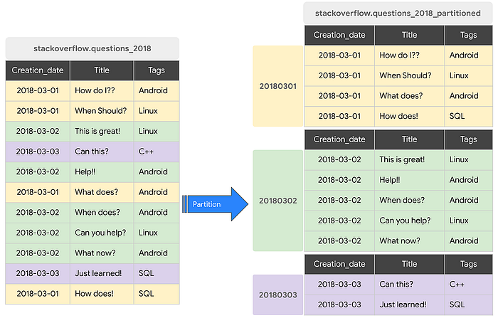

The query above gives you a quick view of how the partitions look like your table. Note that the partition limit is 4000. The figure below shows how the partitioning in BQ looks like

Clustering

Clustering is another technique to cut down processing time by querying on the right chunk of data. Achieved by selecting the columns used to colocate the related data, up to 4 columns can be chosen for clustering. The order of the columns is important as it kind of sorting out the order of the data. For instance, kindly refer to the figure below which the dataset is first partitioned using the date column and then clustered by Tags. In regards to this, it significantly improves the curing time of filter queries as well as aggregate queries. However, it is important to note that it doesn’t show significant improvement in partitioning and clustering if the table is sized below 1GB. Clustering columns must be top-level, non-repeated columns. The available data types for clustering include DATE, BOOL , GEOGRAPHY , INT64 , NUMERIC , BIGNUMERIC , STRING , TIMESTAMP , DATETIME .

Taking the example used in the module, the partitioning and clustering can be performed together as follows:

-- Creating a partition and cluster table
CREATE OR REPLACE TABLE de-zoomcamp-412301.ny_taxi.yellow_tripdata_partitoned_clustered
PARTITION BY DATE(pickup_date)
CLUSTER BY VendorID AS
SELECT * FROM de-zoomcamp-412301.ny_taxi.external_yellow_tripdata_corrected;

In result of that, the total byte of query has been cut down from 1.1GB to 864.5MB of data in Table.

-- Query scans 1.1 GB
SELECT count(*) as trips
FROM de-zoomcamp-412301.ny_taxi.yellow_tripdata_partitoned
WHERE DATE(pickup_date) BETWEEN '2019-06-01' AND '2020-12-31'
  AND VendorID=1;

-- Query scans 864.5 MB
SELECT count(*) as trips
FROM de-zoomcamp-412301.ny_taxi.yellow_tripdata_partitoned_clustered
WHERE DATE(pickup_date) BETWEEN '2019-06-01' AND '2020-12-31'
  AND VendorID=1;

Partitioning vs Clustering

Although clustering and partitioning can be used concurrently. However, there are still differences to be noted when designing and performing our queries

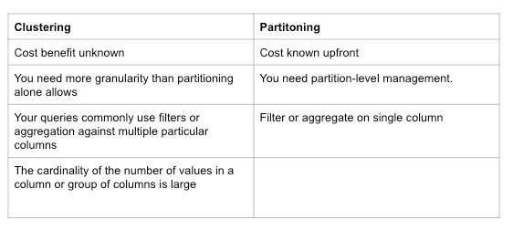
Clustering might be favoured in a few conditions:

When the partitioning results in a small amount of data per partition (less than 1GB)
Partitioning results in a large number of partitioned tables, exceeding 4000
Partitioning results in your mutation operations modifying the majority of partitions in the table frequently (every few minutes).

Aside from that, BigQuery adopted automatic re-clustering. When new data is added to the clustered table, it performs the automatic re-clustering in the background to restore the sort property of the table and the newly inserted data can be written to blocks that contain key ranges that overlap with it previously written blocks. For partitioned tables, re-clustering is down within the scope of each partition.

Internal Infrastructure of BigQuery

It is not necessary to know the internal structure of BigQuery, but it might give us a more intuitive way to understand how our query is being executed behind the scenes. In general, BigQuery is composed of 4 main parts, namely Colossus, Jupiter, Dremel and Borg

Colossus: A cheap storage that stores data in a columnar format that is separated from the compute cluster.
Jupiter: A Google in-house network to connect between Colossus and the compute engine with a 1TiB network speed, ensuring low latency.
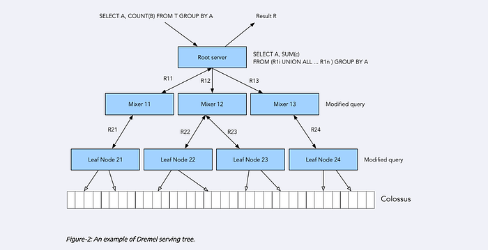
Dremel: Query execution engine, which divides a query into a tree structure, thus each node can execute an individual subset of the query.
Borg: an orchestration solution that handles everything.

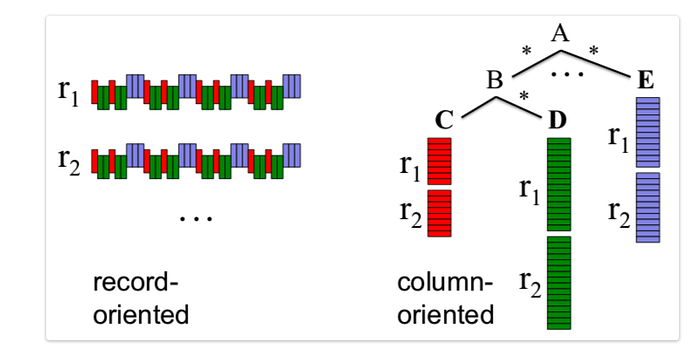
Comparing column-oriented and record-oriented storage, both of them serve different purposes in data science. In the record-oriented storage, it is more likely to be in a .csv file structure which every new line is the new record for an observation. It is relatively easy to understand. In contrast, the column-oriented storage. The data is stored in columns rather than rows. It is very beneficial for query efficiency as it allow us to discard right away the columns that we’re not looking file, reducing the amount that we have to process.

In Dermel, the SQL query engine will take in a query, and then further divide the query into the mixer where the query is modified and brought to a leaf node. At leaf nodes, this is the layer which connects to the colossus to fetch the data for appropriate operation on top of that, then returns to the mixer, then the root server where data is aggregated and returned to the user.